Tofts model#
Show code cell source
# import statements
import os
import numpy as np
from matplotlib import pyplot as plt
import csv
import pandas as pd
import seaborn as sns
from plotting_results_nb import plot_bland_altman, bland_altman_statistics, make_catplot
import json
from pathlib import Path
Test data#
The QIBA DRO data was used for testing of the Tofts model.
Version: QIBA_v11_Tofts from MR Modality Datasets/Dynamic Contrast Enhanced (DCE) MRI/DCE-MRI DRO Data and Code/DCE-MRI DRO Data (Daniel Barboriak) /QIBA_v11_Tofts/QIBA_v11_Tofts_GE/T1_tissue_500/DICOM_dyn
Test case labels: test_vox_T{parameter combination}_{SNR}, e.g. test_vox_T5_30
To get the high SNR dataset, data was averaged as follows:
datVIF = data[:, :9, :]
datVIF = np.mean(datVIF, axis=(0, 1))
datT1 = np.mean(data[44:49, 13:18, :], (0, 1))
datT2 = np.mean(data[32:37, 21:26, :], (0, 1))
datT3 = np.mean(data[42:47, 23:28, :], (0, 1))
datT4 = np.mean(data[22:27, 32:37, :], (0, 1))
datT5 = np.mean(data[22:27, 43:48, :], (0, 1))
Noise was added to the high-SNR data to obtain data at different SNRs. SNR-levels of 20, 30, 50, and 100 were included.
A delayed version of the test data was created by shifting the time curves with 5 time points. This data is labeled as ‘delayed’ and only used with the models that allow the fitting of a delay.
The DRO data are signal values, which were converted to concentration curves using dce_to_r1eff from welcheb/pydcemri from David S. Smith
Input values and reference values were found from the accompanying pdf document, which describes the values per voxel.
T1 blood of 1440
T1 tissue of 500
TR=5 ms
FA=30
Hct=0.45
Tolerances
\(v_e\): a_tol=0.05, r_tol=0, start=0.2, bounds=(0,1)
\(K^{trans}\): a_tol=0.005, r_tol=0.1, start=0.6, bounds=(0,5), units [/min]
delay: a_tol=0.5, r_tol=0, start=0, bounds=(-10,10), units [s]
source: https://qibawiki.rsna.org/images/1/14/QIBA_DRO_2015_v1.42.pdf and https://qidw.rsna.org/#collection/594810551cac0a4ec8ffe574/folder/5e20ccb8b3467a6a9210e9ff
Visualize test data#
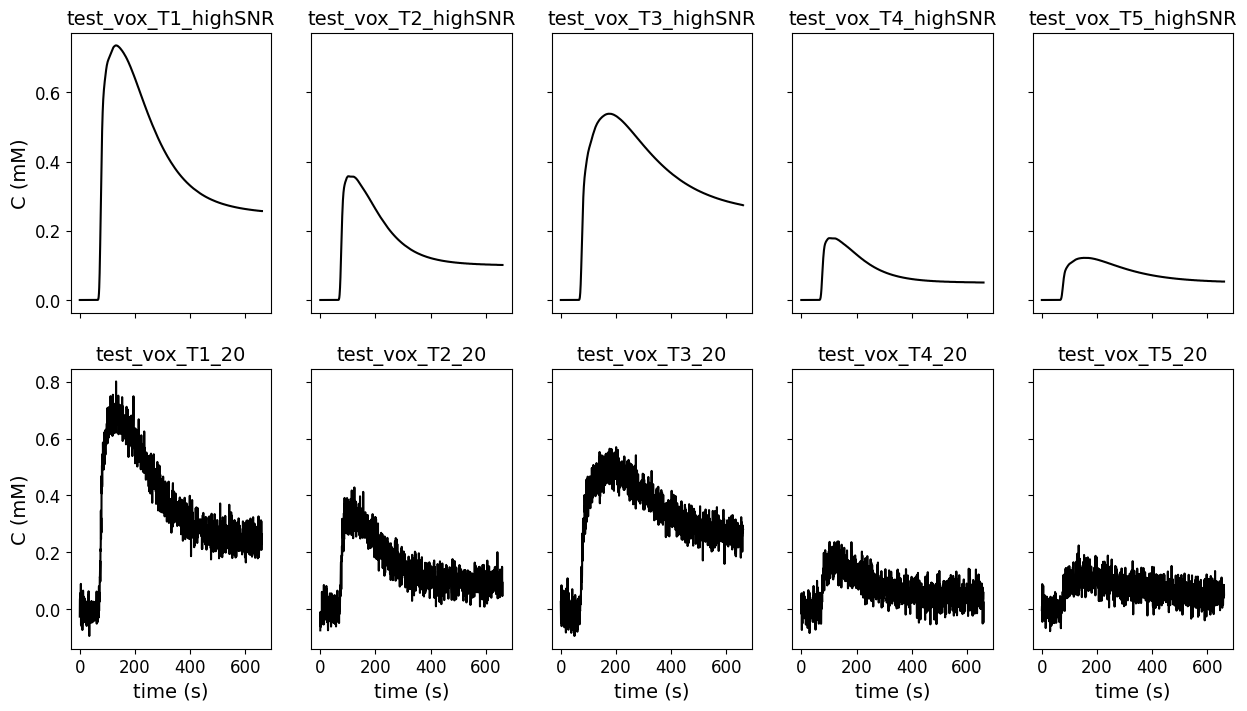
To get an impression of the test data that was used for the Tofts model, below we show the concentration time curves that were the input for the models.
Here we show the data from high SNR from the original (first row) DRO and lowest SNR (SNR = 20; second row).
#plot test data. Load csv file of the test data.
filename = ('../test/DCEmodels/data/dce_DRO_data_tofts.csv')
# read from CSV to pandas
df1 = pd.read_csv(filename)

fig, ax = plt.subplots(2, 5, sharex='col', sharey='row', figsize=(15,8))
for currentvoxel in range(5):

    # first row is high SNR data
    labelname = 'test_vox_T' + str(currentvoxel+1) + '_highSNR'
    testdata = df1[(df1['label']==labelname)]
    t = testdata['t'].to_numpy()
    t = np.fromstring(t[0], dtype=float, sep=' ')
    c = testdata['C'].to_numpy()
    c = np.fromstring(c[0], dtype=float, sep=' ')
    ax[0,currentvoxel].plot(t, c, color='black', label='highSNR')
    ax[0,currentvoxel].set_title(labelname, fontsize=14)
    if currentvoxel ==0:
        ax[0,currentvoxel].set_ylabel('C (mM)', fontsize=14)
    ax[0,currentvoxel].tick_params(axis='x', labelsize=12)
    ax[0,currentvoxel].tick_params(axis='y', labelsize=12)


    # second row is data with SNR of 20
    labelname = 'test_vox_T' + str(currentvoxel+1) + '_20'
    testdata = df1[(df1['label']==labelname)]
    t = testdata['t'].to_numpy()
    t = np.fromstring(t[0], dtype=float, sep=' ')
    c = testdata['C'].to_numpy()
    c = np.fromstring(c[0], dtype=float, sep=' ')
    ax[1,currentvoxel].set_title(labelname, fontsize=14)
    ax[1,currentvoxel].plot(t, c, color='black', label='SNR 20')
    ax[1,currentvoxel].set_xlabel('time (s)', fontsize=14)
    if currentvoxel ==0:
        ax[1,currentvoxel].set_ylabel('C (mM)', fontsize=14)
    ax[1,currentvoxel].tick_params(axis='x', labelsize=12)
    ax[1,currentvoxel].tick_params(axis='y', labelsize=12)
Import data#
Import the csv files with test results. The source data are labelled and the difference between measured and reference values was calculated.
# Load the meta data
meta = json.load(open("../test/results-meta.json"))
# Loop over each entry and collect the dataframe
df = []
for entry in meta:
    if (entry['category'] == 'DCEmodels') & (entry['method'] == 'tofts') :
        fpath, fname, category, method, author = entry.values()
        df_entry = pd.read_csv(Path(fpath, fname)).assign(author=author)
        df.append(df_entry)

# Concat all entries
df = pd.concat(df)
# split delayed and non-delayed data
df['delay'] = df['label'].str.contains('_delayed')

# label data source
df['source']=''
df.loc[df['label'].str.contains('highSNR'),'source']='high SNR'
df.loc[df['label'].str.contains('_20'),'source']='SNR 20'
df.loc[df['label'].str.contains('_30'),'source']='SNR 30'
df.loc[df['label'].str.contains('_50'),'source']='SNR 50'
df.loc[df['label'].str.contains('_100'),'source']='SNR 100'

# label voxels
df['voxel']=''
df.loc[df['label'].str.contains('test_vox_T1'),'voxel']='voxel 1'
df.loc[df['label'].str.contains('test_vox_T2'),'voxel']='voxel 2'
df.loc[df['label'].str.contains('test_vox_T3'),'voxel']='voxel 3'
df.loc[df['label'].str.contains('test_vox_T4'),'voxel']='voxel 4'
df.loc[df['label'].str.contains('test_vox_T5'),'voxel']='voxel 5'

author_list = df.author.unique()
no_authors = len(author_list)

# calculate error/difference between measured and reference values
df['error_Ktrans'] = df['Ktrans_meas'] - df['Ktrans_ref']
df['error_ve'] = df['ve_meas']- df['ve_ref']

# tolerances
tolerances = { 'Ktrans': {'atol' : 0.005, 'rtol': 0.1 },'ve': {'atol':0.05, 'rtol':0}, 'delay': {'atol' : 0.5, 'rtol': 0 }}
Results#
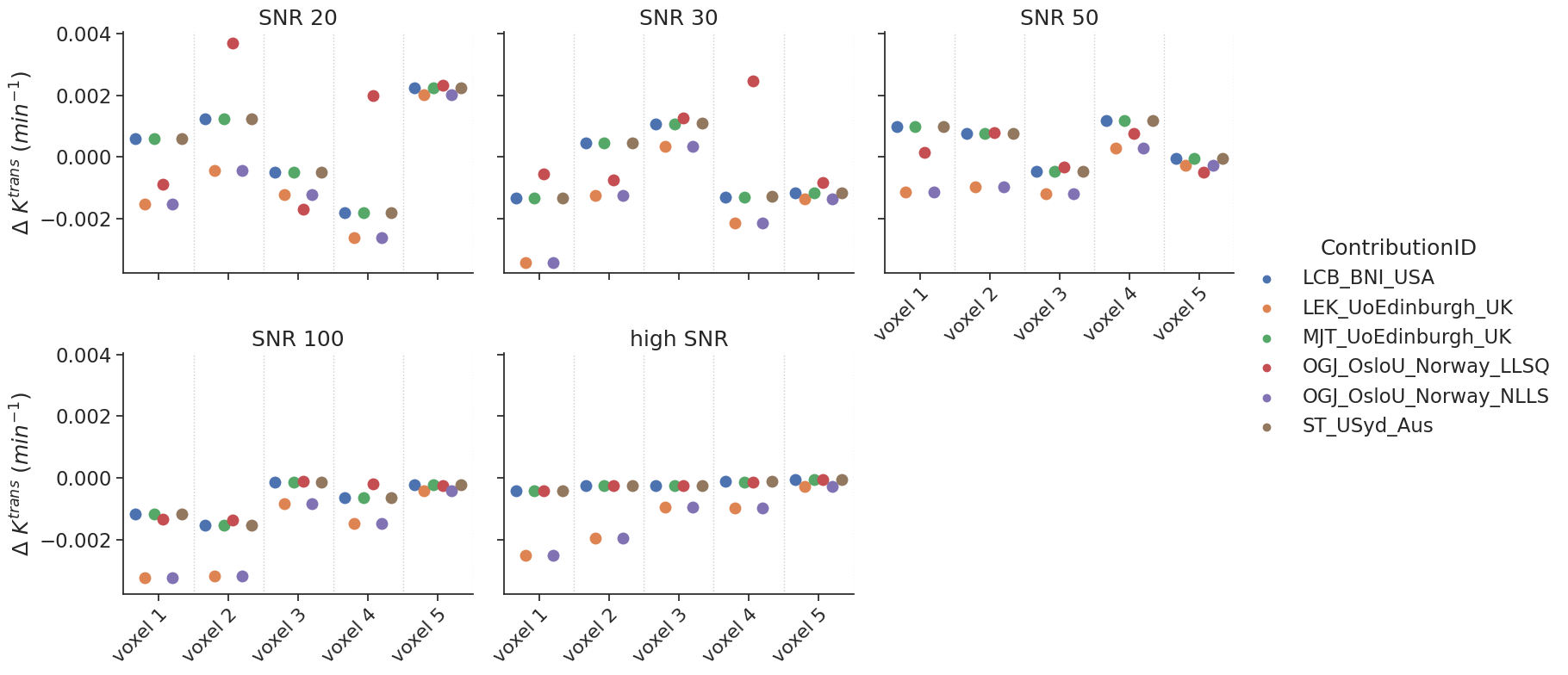
Non-delayed results#
Some models allow the fit of a delay. For the tests with non-delayed data, the delay was fixed to 0. The data are shown with a categorial swarm plot, so for each text voxel separately to better appreciate the differences between contributions. Note that, the x-axis is not a continuous axis, but has a label per test voxel. To get an idea of the reference values per test case, the table below refers as a legend for the figure.
Note that, one author (OGJ_OsloU_Norway) provided two options to fit the model (LLSQ and NLLS). These were considered separate contributions.
df.head(n=5)[['voxel','Ktrans_ref','ve_ref']]
| voxel | Ktrans_ref | ve_ref | |
|---|---|---|---|
| 0 | voxel 1 | 0.35 | 0.5 |
| 1 | voxel 2 | 0.20 | 0.2 |
| 2 | voxel 3 | 0.20 | 0.5 |
| 3 | voxel 4 | 0.10 | 0.1 |
| 4 | voxel 5 | 0.05 | 0.1 |
Show code cell source
# set-up styling for seaborn plots
sns.set(font_scale=1.5)
#sns.set_style("whitegrid")
sns.set_style("ticks")
plotopts = {"hue":"author",
            "col":"source",
            "col_order":["SNR 20","SNR 30","SNR 50","SNR 100","high SNR"],
            "dodge":True,
            "col_wrap":3,
            "s":100,
            "height":4,
            "aspect":1.25
           }
# Instead of a regular bland-altman plot we opted for a catplot + swarm for these results.
# In this way we can appreciate the results of the different contributions per test case better.
# The downside is that the values of the test cases are not obvious. This might be something to improve upon at a later stage

make_catplot(x='voxel', y="error_Ktrans", data=df[~df['delay']],
             ylabel="$\Delta$ $K^{trans}$ ($min^{-1}$)", **plotopts)
# same for v_e
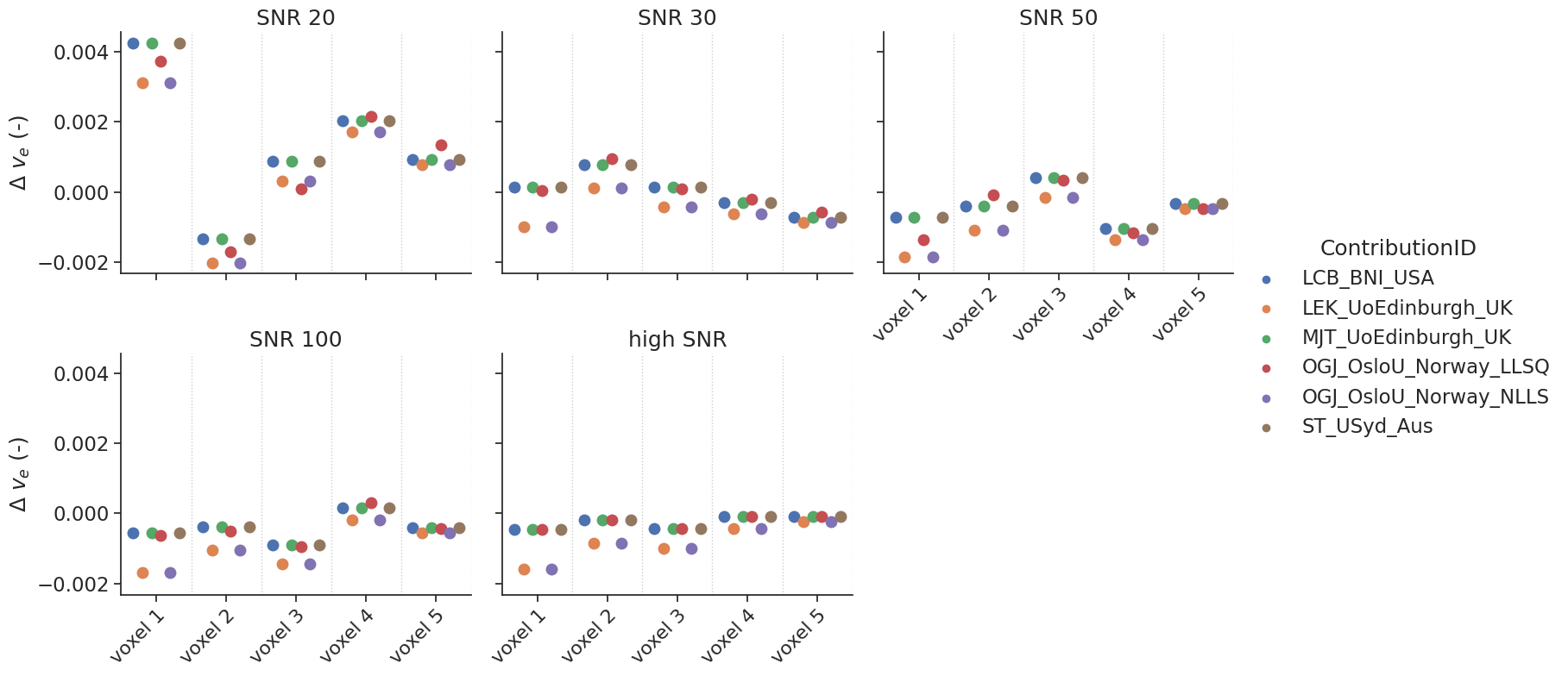
make_catplot(x='voxel', y="error_ve", data=df[~df['delay']],
ylabel="$\Delta$ $v_{e}$ (-)", **plotopts)
Bias results estimated \(K^{trans}\) values combined for all voxels and all SNR levels
resultsBA = bland_altman_statistics(data=df[~df['delay']],par='error_Ktrans',grouptag='author')
print(resultsBA)
                           bias     stdev  LoA lower  LoA upper
author
LCB_BNI_USA           -0.000112  0.000994  -0.002061   0.001837
LEK_UoEdinburgh_UK    -0.001222  0.001230  -0.003632   0.001188
MJT_UoEdinburgh_UK    -0.000114  0.000995  -0.002064   0.001835
OGJ_OsloU_Norway_LLSQ  0.000145  0.001305  -0.002412   0.002702
OGJ_OsloU_Norway_NLLS -0.001222  0.001230  -0.003632   0.001188
ST_USyd_Aus           -0.000110  0.000994  -0.002059   0.001839
Bias results estimated \(v_e\) values combined for all voxels and all SNR levels
resultsBA = bland_altman_statistics(data=df[~df['delay']],par='error_ve',grouptag='author')
print(resultsBA)
                           bias     stdev  LoA lower  LoA upper
author
LCB_BNI_USA            0.000052  0.001132  -0.002166   0.002270
LEK_UoEdinburgh_UK    -0.000518  0.001130  -0.002733   0.001697
MJT_UoEdinburgh_UK     0.000053  0.001132  -0.002166   0.002271
OGJ_OsloU_Norway_LLSQ -0.000014  0.001126  -0.002221   0.002193
OGJ_OsloU_Norway_NLLS -0.000518  0.001130  -0.002733   0.001697
ST_USyd_Aus            0.000052  0.001132  -0.002166   0.002271
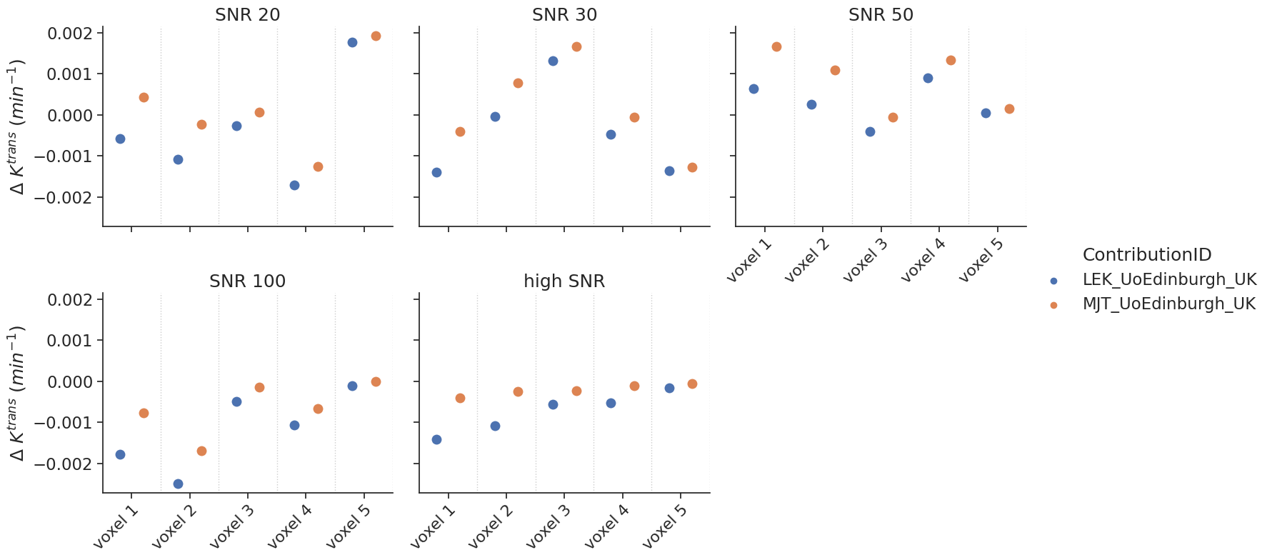
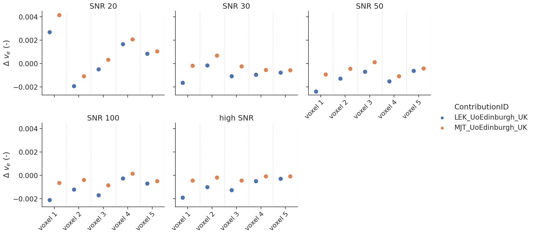
Delayed results#
Some contributions allowed the fitting of a delay. For those, additional tests with a delay were performed.
make_catplot(x='voxel', y="error_Ktrans", data=df[df['delay']],
             ylabel="$\Delta$ $K^{trans}$ ($min^{-1}$)", **plotopts)
make_catplot(x='voxel', y="error_ve", data=df[df['delay']],
             ylabel="$\Delta$ $v_{e}$ (-)", **plotopts)
resultsBA = bland_altman_statistics(data=df[df['delay']],par='error_Ktrans',grouptag='author')
print(resultsBA)
                        bias     stdev  LoA lower  LoA upper
author
LEK_UoEdinburgh_UK -0.000481  0.000994  -0.002429   0.001467
MJT_UoEdinburgh_UK  0.000058  0.000925  -0.001755   0.001871
resultsBA = bland_altman_statistics(data=df[df['delay']],par='error_ve',grouptag='author')
print(resultsBA)
                        bias     stdev  LoA lower  LoA upper
author
LEK_UoEdinburgh_UK -0.000772  0.001149  -0.003024   0.001481
MJT_UoEdinburgh_UK -0.000024  0.001109  -0.002198   0.002150
Notes#
Some contributions included only the forward model, no fitting routine. For those cases we used the curvefit module from scipy package to estimate the output parameters. In all other cases the contributed fitting routine was included.